Novelty
- Propose an ESDF free path planner
Methodology
Collision Avoidance Force Estimation
B-spline control points → Q B-spline initiated regardless of collision (straight line leading to the goal point) →
Generate a collision free path Γ for each colliding segment. Each control point Q will be assigned an anchor point . is at the surface of the obstacle Repulsive direction vectors from Q to
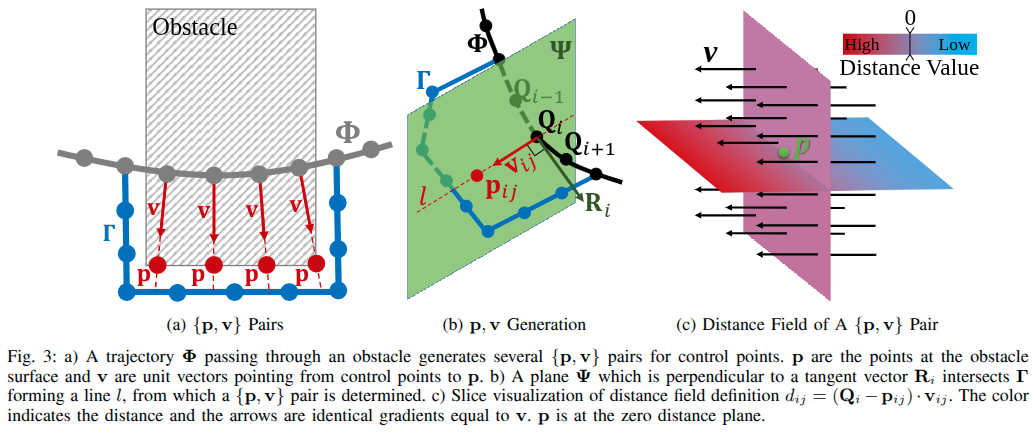
The obstacle distance from to the jth obstacle is defined as

Note : Each {p,v} pair belongs to one specific control point
Algorithm for {p,v} pair assignment
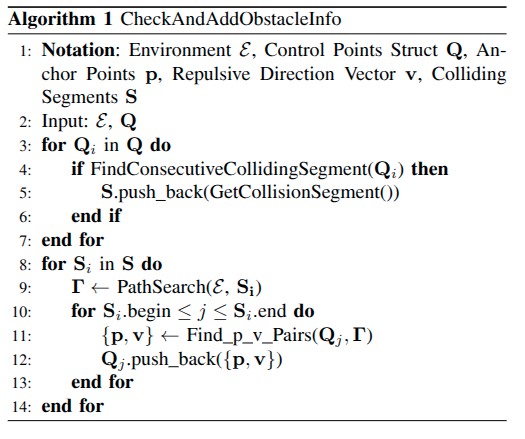
To prevent duplication of {p,v} pair before the trajectory exits the obstacle, if is inside the obstacle then the obstacle is termed as a newly discovered ie. for all j. Allows for only necessary obstacles to contribute to trajectory → reduces operation time.
THE PROBLEM WITH ESDFs.. Lead to local minimums→ fail to escape, need a collision free initial trajectory to prevent getting stuck into local minimums
Gradient Based Trajectory Optimization
Formulation
Trajectory is defined using B-spline() and all respective parameters.
Uniform B-spline is used here.
Convex Hull Property & kth derivative property of B-spline is used similar to FAST-Planner
 Control points for Velocity, Acceleration, Jerk based on the kth derivative property of B-spline.
Note:
Drone system here is used in the reduced Differentially Flat Output space. Normally drone operates in a 12 dimensional state space. We map it to a 4 dimensional space. Differentially Flat: The quadrotor dynamics can be written as a function of selected flat output and their derivatives. (https://ieeexplore.ieee.org/document/5980409)
The optimization problem can be modelled as:
 where Js is the smoothness penalty, Jc is for collision, and Jd indicates feasibility. λs, λc, λd are weights for each penalty terms.
-
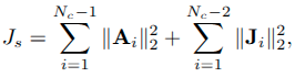
Smoothness Penalty (Js) : Benefits from the convex hull property, minimising the control points of 2nd and 3rd order derivatives of B-spline.
-
Collision Penalty (Jc) :
Pushes control points away from obstacles. Adopts a safety clearance of sf and punishes dij < sf.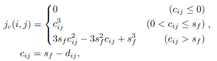 Computed per control point Qi. Cost of each Qi is accumulated for all corresponding {p,v} pairs so,
 and
and 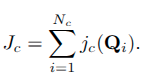 Calculates the gradient required as a mathematical operation. Normally ESDF will be calculated and stored in the memory and then looked up. The algorithm here calculates gradient as a derivative of Jc.
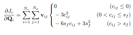 (Reduces trajectory computation time since memory lookup for ESDF array is much more time consuming than just calculating the gradient on spot)
 -
Feasibility Penalty (Jd): Feasibility check on each higher order derivative of the B-spline trajectory.
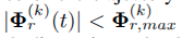 for all t and

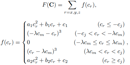 F() is twice continuously differentiable. where cr ∈ C ∈ {Vi, Ai, Ji}, a1, b1, c1, a2, b2, c2 are chosen to meet the second-order continuity, cm is the derivative limit,cj is the splitting points of the quadratic interval and the cubic interval. λ < 1 − is an elastic coefficient with 1 to make the final results meet the constraints, since the cost function is a tradeoff of all weighted terms.
Numerical Approximation
- For the objective function J mentioned above a Hessian Matrix is approximated per obstacle.
- Since calculation of the Hessian is not possible on the fly, Quasi Newton methods are used, in this case L-BFGS.
- The solver also needs to be able to compute the Hessian for new incoming obstacles, maintain memory constrains, drop the the old Hessian once a new obstacle comes.
Time Re Allocation and Trajectory Equation
Simplified idea is that just as FAST-Planner and similar planners changed the from uniform to non uniform B-spline. That may lead to a domino effect leading to change in the trajectory.
EGO Planner uses the L-BFGS optimisation to move the new trajectory closer to the initial obstacle avoidance trajectory.
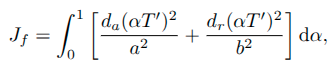
The is scaled using 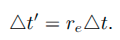
 .
.
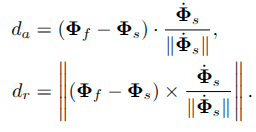
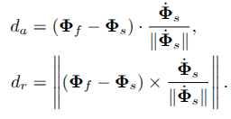
The optimisation is performed on the following function
 where
where